Line Following

Because of mechanical design constraints, we needed to be able to accurately and quickly follow a line using four tape sensors all placed along the axis between the two motors. The tape sensors were designed so that the middle two would follow over the line and the other two would be used to detect bends or tape ends. To better control the robot, we created a basic MATLAB model of line following. This led to a simple line following control where we calculate the difference between left and right wheel speeds as dv using the following control law.

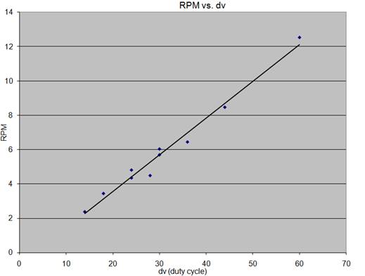
Where x is the estimate of distance error from the line

Theta is the estimate of attitude error.

The idea of the controller is to minimize and eventually eliminate overshoot and oscillation where the robot continuously bounces from one side of the line to another. If the robot loses the line, as it returns to the tape, it should be attempting to straighten out instead of continuing onto the line and then past it again. We approximated distance error by looking at the two middle tape sensors. If both were on the line, x=0; if only the left was on the line, x=1; if only the right was on the line, x=-1; and if neither were on the line, x=+/-2, depending on which sensor did see the line last. To estimate theta, we needed to know how the robot would turn when given different inputs to the two motors. We ran some simple tests at various duty cycles to produce the following plot that shows that the RPM of the robot varies roughly linearly with dv and has a y-intercept very close to 0. RPM was measured by timing the robot through a set number of revolutions.

We could then propagate theta using dv and the time interval dt. However, since we have no way at guessing our initial value of theta, we implemented slight decay onto the previous theta estimate. This form of line following closely approximates a PI (Proportional Integral) control, but also works to “lose” erroneous histories in the integrator. This produced the discrete theta estimator:

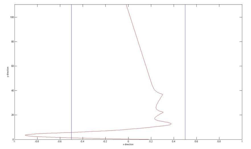
Where ω is derived from the linear estimate of ω vs. dv

Modeled in MATLAB, this controller fared far better than simple left-right control using the current state of the tape sensors and produced the plot shown below. Note that the distance and control units used are relative, and are not necessarily accurate to the robot. Note, however, that despite significant initial heading error, the controller is able to always move forward and rapidly straighten out on the line. The x and y axis have significantly different scales, so the actual path travelled is much straighter than it may seem.

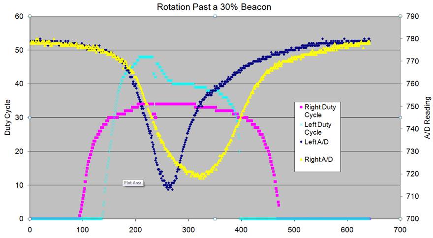
Since we wanted to always move forward, after calculating dv from the control law above, we used the sign of dv to determine which wheel should be driven slower and then subtracted dv from a base duty cycle (we used 40% as max duty). Furthermore, since we did not want to actually spin in place (which might never bring the tape sensors back to the line), we made the minimum duty cycle for either motor 0 (which mean that the wheel would never drive backward). This overall control law was a success and was very effective at following continuous tape lines at high speeds, provided one of the outside tape sensors did not malfunction and cause the robot to think it was at the end of the tape. Line following was used in our program to guide the robot to the ball dispenser—the robot followed the black tape first to the 90 degree elbow, and then followed the line backwards to the dispenser.

Beacon Targeting

As described in the Electrical Design section, our beacon sensors are used to provide two different signals. Rising and falling edges are measured to provide duty cycle from each of the two eyes but also, a low pass filter gives an analog estimate of signal strength. To assess the usefulness of these two signals, we spun in place at various points on the board and took data through both left and right sensors. The plot below is an example of one such plot.

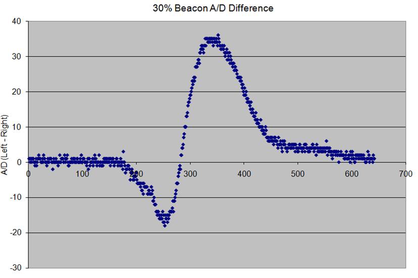
Note that the duty cycle plots are fairly accurate (although significantly different between the two sensors) when pointed at the beacon, but there are fall off regions at the edges of each sensors vision. We were, however, able to consistently use the duty cycles measured to target the proper beacon from the required spots on the board. The plot below shows the difference in the analog signals from the two sensors. Once the robot was aimed toward a beacon, we used this difference to accurately charge towards the beacon. The overall control used here is a simplified version of the line following where

Like the line following algorithm, we scaled the duty cycles between a maximum duty (40%) and a minimum of zero, to prevent the robot from getting stuck swiveling in place. Duty cycle measurements from the two sensors were used to rotate in place and target a beacon and the differential A/D controller was used while the robot moved towards (and eventually over) Goal 3. This simple targeting system proved surprisingly accurate and reliable during testing.